Neural Radiance Field (NeRF)

Goal: Represent a continuous 3D scene as a fully-connected neural network and synthesize novel views of the scene.

Contribution: Presents the first continuous neural scene representation that is able to render high-resolution photorealistic novel views of real objects and scenes from RGB images captured in natural settings.

Concept

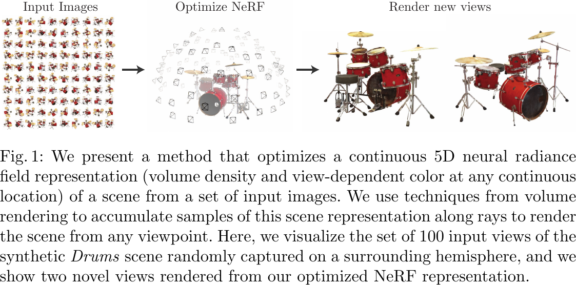
Synthesize novel views from a set of input images, from Figure 1 of Mildenhall et al., 2020.

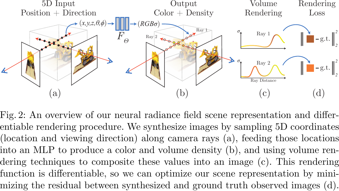
An overview of the NeRF scene representation and differentiable rendering procedure, from Figure 2 of Mildenhall et al., 2020.

1. Parameterizing the NeRF

The MLP network $\F:(\xyz, \thetaphi)\to(\rgb,\density)$ is a 5D neural radiance field that represents a continuous scene as the volume density and directional emitted radiance at any point in space.

Input a 3D location $\x=\xyz$, and a 2D viewing direction $\thetaphi$ which is converted to a 3D Cartesian unit vector $\d$ during rendering.
Output an emitted color $\c=\rgb$, and a volume density $\density$.
$\density$ should not be dependent of the viewing direction $\d$, so as to achieve multiview consistency.

A differentiable algorithm is needed to synthesize a novel view (a RGB image) from $\F$ for training/inference.

2. Volume Rendering

Perform (differentiable) volume rendering based on $\F$ to render novel views as 2D projections.

Surface Rendering vs. Volume Rendering
- Surface Rendering: Loop through geometric surfaces and check for ray hits.
- Volume Rendering: Loop through ray points and query geometry.
The volume density $\density(\x)$ can be interpreted as the differential probability of a ray terminating at an infinitesimal particle at location $\x$.
- Probabilistic modeling enables the representation of translucent or transparent objects.
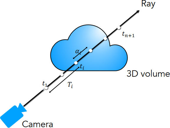
Given a camera ray $\r(\t)=\o+\t\d$ (starting from its origin $\o$) with near and far bounds $\tnear$ and $\tfar$, its expected color $\C(\r)$ is: $$ \C(\r) = \int_{\tnear}^{\tfar}\T(\t)\density(\t)\c(\t,\d)dt, $$ where $\T(\t)=\exp\left(-\int_{\tnear}^{\t}\density(s)ds\right)$, $\density(\t)=\density(\r(\t))$, and $\c(\t,\d)=\c(\r(\t),\d)$.

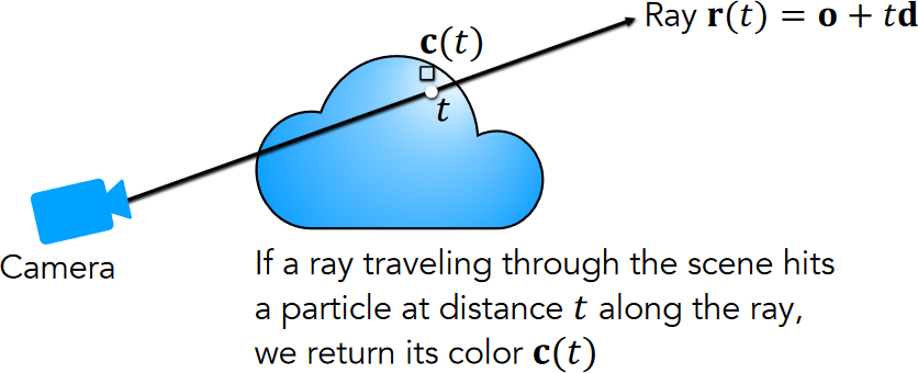
Volumetric formulation for NeRF, from p.98 of UC Berkeley CS194-26, Neural Radiance Fields 1.
- $\Pr(\text{no hit before }\t) = \T(\t)$ denotes the accumulated transmittance along the ray from $\tnear$ to $\t$, i.e., the probability that the ray travels from $\tnear$ to $\t$ without hitting any other particle.
- $\Pr(\text{hit at }\t) = \density(\t)dt$ denotes the probability that the ray hits a particle in a small interval around $\t$.
- Since $\Pr(\text{first hit at }\t) = \Pr(\text{no hit before }\t)\times\Pr(\text{hit at }\t) = \T(\t)\density(\t)dt$, we can derive the expected color $\C(\r)$ by integrating the probabilities of hitting each particle times its emitted color.
- Based on the probability fact that: $$ \Pr(\text{no hit before }\t+dt) = \Pr(\text{no hit before }\t)\times\Pr(\text{no hit at }\t) $$$$ \Rightarrow \T(\t+dt) = \T(\t)\times(1-\density(\t)dt), $$ we can solve $\T(\t)$ within a few steps.
  Derivation Sketch
  
  The derivation of $\T(\t)$ is based on the following steps: ¹²
  1. Rearrange the equation and derive: $\T'(\t)=-\T(\t)\cdot\density(\t)$.
  2. Rearrange
  3. Integrate
  4. Exponentiate
- However, $\C(\r)$ is intractable.

Esimate $\C(\r)$ with quadrature by partitioning $[\tnear, \tfar]$ into $N$ segments with endpoints $\{\t_1, \t_2, \dots, \t_{n+1}\}$ and length $\delta_i=\t_{i+1}-\t_i$.

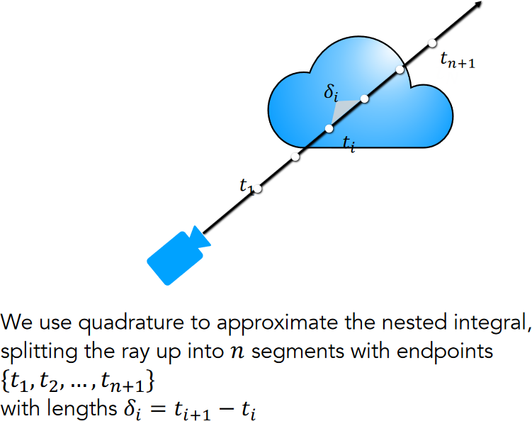
Approximating the nested integral, from p.114 of UC Berkeley CS194-26, Neural Radiance Fields 1.
- Assume each segment has constant volume density $\density_i$ and color $\c_i$.
- Based on the assumptions, derive $\T(\t)$ for $\t\in[\t_i,\t_{i+1}]$:
  
  \[\begin{aligned} \T(\t)&=\T(\t_1 \rightarrow \t_i) \cdot \T(\t_i \rightarrow \t)\\ &=\exp\left(-\int_{\t_1}^{\t_i}\density_i ds\right) \exp\left(-\int_{\t_i}^{\t}\density_i ds\right)\\ &=\T_i \exp(-\density_i(\t - \t_i)),\\ \end{aligned}\]
  
  where $\displaystyle \T_i=\exp\left(-\sum_{j=1}^{i-1}\density_j\delta_j\right)$.
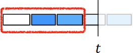
  - $\Pr(\text{no hit within }[\t_1, \t_i]) = \T_i$ is the transmittance within $[\t_1, \t_i]$.
    
    How much light is blocked by all previous segments? from p.120-122 of UC Berkeley CS194-26, Neural Radiance Fields 1.
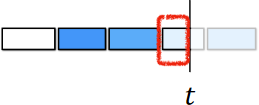
  - $\Pr(\text{no hit within }[\t_i, \t]) = \exp(-\density_i(\t - \t_i))$ is the transmittance within $[\t_i, \t]$.
    
    How much light is blocked partway through the current segment? from p.120-122 of UC Berkeley CS194-26, Neural Radiance Fields 1.
  - Plugin the derived $\T(\t)$ into the original equation of $\C(\r)$:
    
    \[\begin{aligned} \C(\r) &= \int_{\tnear}^{\tfar}\T(\t)\density(\t)\c(\t,\d)dt\\ &\approx \sum_{i=1}^{N}\T_i(1-\exp(-\density_i\delta_i))\c_i:=\hat{\C}(\r) \end{aligned}\]
    Derivation Sketch
    
    The derivation of $\C(\r)$ is based on the following steps: ¹²
    1. Piecewise approximation: $\displaystyle \C(\r) \approx \sum_{i=1}^{N}\int_{\t_i}^{\t_{i+1}}\T(\t)\density_i\c_i dt$.
    2. Substitute
    3. Integrate
    4. Cancel
- However, training with fixed endpoints isn't suitable for learning continuous scene representations.

Apply stratified sampling by partitioning $[\tnear, \tfar]$ into $N$ bins and draw one sample uniformly at random from each bin: $$ \t_i\sim\gU\left[\tnear+\frac{i-1}{N}(\tfar-\tnear), \tnear+\frac{i}{N}(\tfar-\tnear)\right], $$ and use the sampled endpoints to estimate $\C(\r)$.

Connection to alpha compositing by defining alpha values $\alpha_i=1−\exp(−\sigma_i\delta_i)$:

\[ \hat{\C}(\r)=\sum_{i=1}^{N}\T_i\alpha_i\c_i \]

Volume rendering integral estimate, from p.129 of UC Berkeley CS194-26, Neural Radiance Fields 1.
- $\Pr(\text{no hit within }[\t_1, \t_i]) = \T_i$ is the transmittance within $[\t_1, \t_i]$.
- $\Pr(\text{hit within }[\t_i, \t]) = \alpha_i$ is the segment opacity within $[\t_i, \t]$.
- $\Pr(\text{first hit within }[\t_i, \t])$$ = \Pr(\text{no hit within }[\t_1, \t_i])\times\Pr(\text{hit within }[\t_i, \t])$$ = \T_i\alpha_i$,

3. Implementation Details

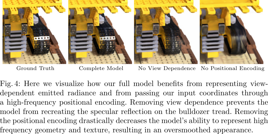
Positional encoding. Maps the inputs to a higher dimensional space using high frequency functions to represent high-frequency scene content, since neural networks are biased towards learning lower frequency functions. ³
Hierarchical volume sampling. Estimate the volume PDF along a ray with an additional coarse network $F_{\Theta_c}$ and sample from it to allocate samples proportionally to their expected effect on the final rendering. This improves training efficiency by avoiding repeatedly sampling free space and occluded regions that do not contribute to the rendered image/pixel.
- Two networks, a coarse network $F_{\Theta_c}$ and a fine network $F_{\Theta_f}$, are jointly trained.
  - $F_{\Theta_c}$ enables sampling from regions which are expected to contain visible content.
  - $F_{\Theta_f}$ is the main network that renders the final image during inference.
For each ray:
- Sample a first set of $N_c$ locations with stratified sampling, and evaluate them on the coarse network $F_{\Theta_c}$ to compute $(T_i, \alpha_i, \c_i)$ and the coarsely rendered pixels.
  - The expected color of the coarse network can be computed by $\Ccoarse(\r;\Theta_c)$$ = \sum_{i=1}^{N_C}\T_i\alpha_i\c_i = \sum_{i=1}^{N_C}w_i\c_i$, where $w_i=\T_i\alpha_i$.
- $\Pr(\text{hit within }[\t_i, \t_{i+1}]) \approx \hat{w}_i = w_i / \sum_{j=1}^{N_C} w_j$ is a piecewise constant approximation of the volume PDF along the ray by normalizing $w_i$.
  - The normalization is required since each segment along the ray does not necessarily have constant volume density and color.
- Sample a second set of $N_f$ locations with inverse transform sampling according to the estimated volume PDF, and evaluate all $N_c+N_f$ locations on the fine network $F_{\Theta_f}$ to compute the (finely) rendered pixels based on its expected color $\Cfine(\r;\Theta_f)$.

4. Training

Optimize $\Theta$ for each scene, based on a dataset of captured RGB images of each scene, the corresponding camera poses, intrinsic parameters, and scene bounds.

The camera poses, intrinsics, and bounds of real data is estimated with the COLMAP structure-from-motion package.
At each iteration, sample a batch of camera rays from the set of all pixels in the dataset.
Use hierarchical sampling to query $N_c$ samples from the coarse network and $N_c + N_f$ samples from the fine network for each ray.
Perform (differentiable) volume rendering to render the color of each ray from both sets of samples.
Optimize according to the total squared error between the rendered and the ground truth pixel colors for both the coarse and fine renderings. $$ \gL(\Theta_c,\Theta_f)=\sum_{\r\in\gR}\left[\norm{\Ccoarse(\r;\Theta_c)-\C(\r)}_2^2+\norm{\Cfine(\r;\Theta_f)-\C(\r)}_2^2\right] $$
Discard the coarse network $\Ccoarse$ after training and use the fine network $\Cfine$ for inference.

Experiments

Benchmark

Outperform all prior methods by a wide margin.

Analysis

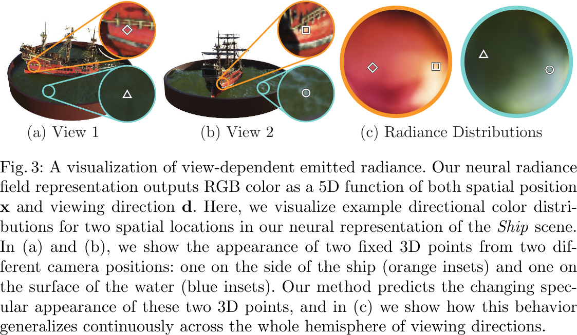
A visualization of view-dependent emitted radiance, from Figure 3 of Mildenhall et al., 2020.

Ablation study, from Figure 4 of Mildenhall et al., 2020.

Official Resources

[ECCV 2020] NeRF: Representing Scenes as Neural Radiance Fields for View Synthesis [arxiv][paper][ link][code][site][video] (citations: 2545, 2408, as of 2023-03-29)

Community Resources

UC Berkeley CS194-26/294-26: Intro to Computer Vision and Computational Photography
- Neural Radiance Fields 1
- Neural Radiance Fields 2

The high-level overview of solving $\T(\t)$ and $\C(\r)$ can be found in p.105-109 and p.123-126 of Neural Radiance Fields 1 from UC Berkeley CS194-26/294-26: Intro to Computer Vision and Computational Photography. ↩↩
The formal derivation of $\T(\t)$ and $\C(\r)$ can be found in Tagliasacchi et al., Volume Rendering Digest (for NeRF), 2022 ↩↩
Rahaman et al., On the Spectral Bias of Neural Networks, ICML 2019 ↩