Low-rank adaptation (LoRA)

Goal: Reduce fine-tuning cost by injecting trainable rank decomposition matrices.

Contribution: Reduce the number of trainable parameters by 10,000 times and the GPU memory requirement by 3 times, while introducing no additional inference latency.

Concept

Hypothesize that the change in weights during model adaptation has a low intrinsic rank.
- For many deep learning tasks with a heavily over-parametrized neural network, the learned neural network will enjoy low-rank properties after training. (Oymak et al., 2019)
For a pre-trained weight matrix $W_{0} \in R^{d \times k}$ , constrain its update $Δ W$ by defining the merged weight matrix as $W_{0} + Δ W = W_{0} + B A$ , where $B \in R^{d \times r}, A \in R^{r \times k}$ , and rank $r ≪ min (d, k)$ .
$A$ is initialized using a Guassian distribution, while $B$ is initialized with zero, such that $Δ W = B A = 0$ at the beginning of fine-tuning.
This study is limited to only adapting the attention weights ( $W_{q}, W_{k}, W_{v}, W_{o}$ ). Adapting other layers such as MLP, LayerNorm, and biases are left for future works.

Architecture of LoRA, from Figure 1 of Hu et al., 2022.

Advantages

A Generalization of Full Fine-tuning. Recovers the expressiveness of full fine-tuning by setting $r = d$ .
No Additional Inference Latency. Pre-compute $W = W_{0} + B A$ before inference. When switching to another downstream task, subtract $B A$ and add $B^{'} A^{'}$ .
Lower hardware requirements. Reduce the number of trainable parameters by 10,000 times and the GPU memory requirement by 3 times.

Still have limitations such as difficulties on batching inputs of different downstream tasks.

Some drawbacks of other fine-tuning methods:

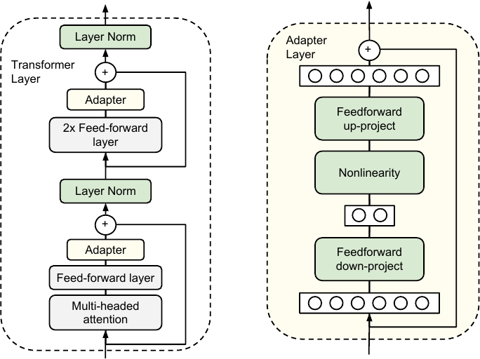
Adapter Layers. Keep the parameters of the pre-trained model frozen. Add two adapter layers per transformer block, and only update these adapter layers during fine-tuning.
- No direct ways to bypass the extra compute in adapter layers.
- The small bottleneck in the adapter layers limits hardware parallelism, increasing latency.
Architecture of the adapter module, from Figure 2 of Houlsby et al., 2019.

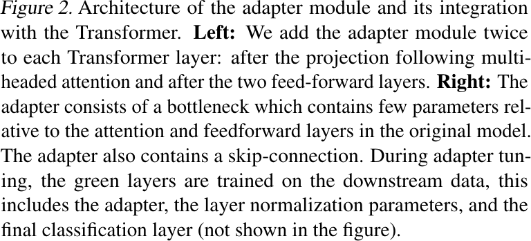
Prefix Tuning. Keep the parameters of the pre-trained model frozen. Prepends a sequence of continuous task-specific vectors (i.e., prefix) to the input sequence, and only update these vectors (i.e., soft prompt) during fine-tuning.
- Difficult to optimize, its performance changes non-monotonically in trainable parameters.
- Reduces the sequence length available for downstream tasks.
Prefix-Tuning, from Figure 1 of Li et al., 2021.

Experiments

Benchmark

Inference Latency, from Table 1 of Hu et al., 2022.

Performance, from Table 4 of Hu et al., 2022.

Analysis

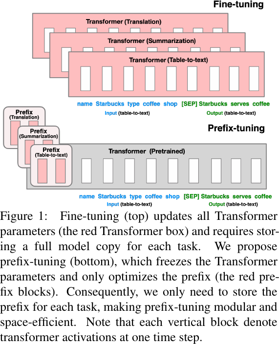
Which weight matrices in Transformer should we apply LoRA to?

Applying LoRA to different types of attention weights, from Table 5 of Hu et al., 2022.

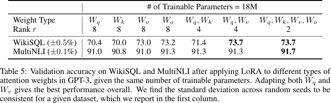
Apply LoRA to $W_{q}, W_{v}$ .
Optimal rank $r$ for LoRA?

Applying LoRA with different ranks, from Table 6 of Hu et al., 2022.

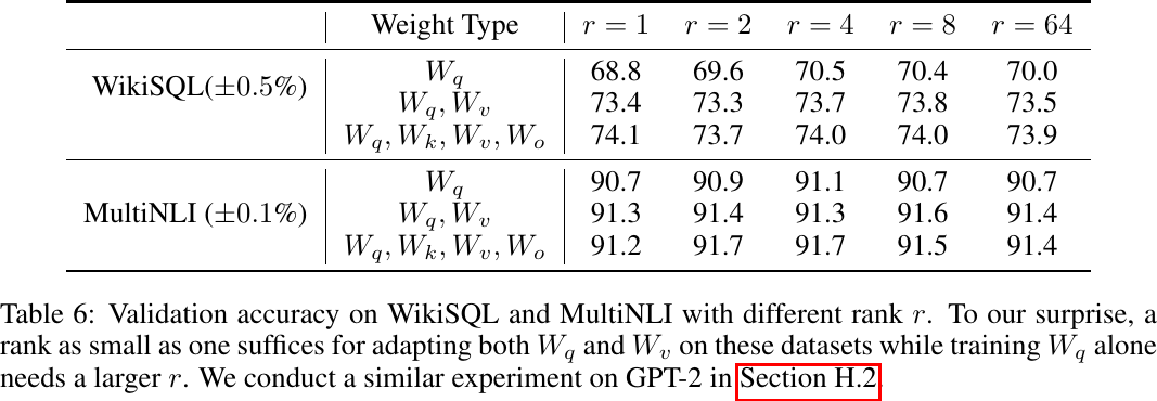
Apply LoRA with $r = 4$ .

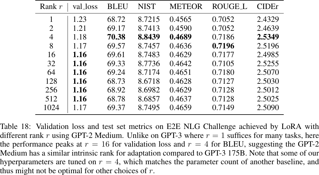
Applying LoRA with different ranks, from Table 18 of Hu et al., 2022.
Does $Δ W$ highly correlate with $W$ ?

Settings:
- Learn adaptation matrices $A_{r = 8}$ and $A_{r = 64}$ with $r = 8$ and $64$ , respectively.
- Perform singular value decomposition (SVD) and obtain the right-singular unitary matrices $U_{A_{r = 8}}$ and $U_{A_{r = 64}}$
- Use Grassmann distance $ϕ (A_{r = 8}, A_{r = 64}, i, j) \in [0, 1]$ to measure how much of the subspace spanned by the top $i$ singular vectors in $U_{A_{r = 8}}$ is contained in the subspace spanned by top $j$ singular vectors of $U_{A_{r = 64}}$
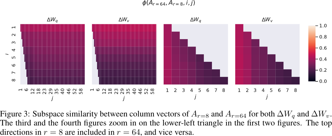
Subspace similarity between $A_{r = 8}$ and $A_{r = 64}$ , from Figure 3 of Hu et al., 2022.

Observations:
- Top singular vector overlap significantly between $A_{r = 8}$ and $A_{r = 64}$ , while others do not.
- These top singular-vector directions are the most useful, while others contain mostly random noises.
- $A_{r = 8}$ and $A_{r = 64}$ share a subspace of dimension 1 with normalized similarity $> 0.5$ , which verifies the experiments that $r = 1$ can still perform quite well.
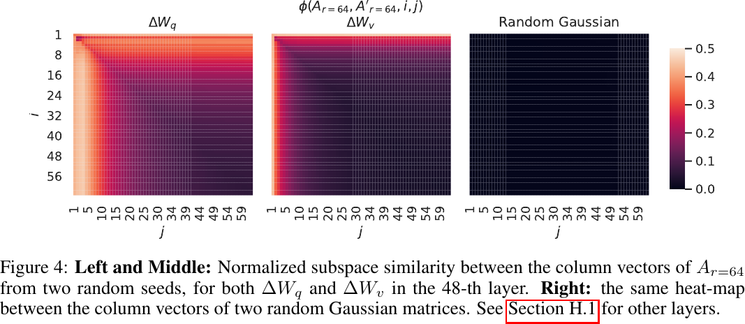
Subspace similarity between two $A_{r = 64}$ fine-tuned with different random seeds, from Figure 4 of Hu et al., 2022.

Observations:
- Similarly, the top singular-vector directions are the most useful, while others contain mostly random noises.
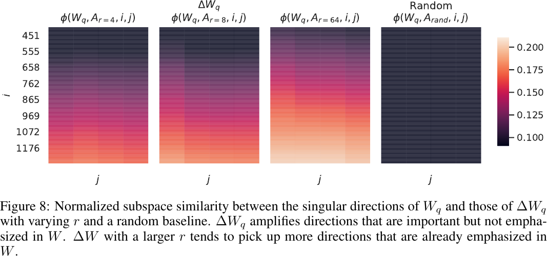
Settings:
- Project $W$ onto the $r$ -dimensional subspace of $Δ W$ .
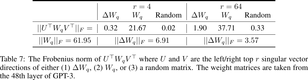
Correlation between $Δ W$ and $W$ and Amplication Factor of $Δ W$ , from Table 7 of Hu et al., 2022.

Observations:
- $Δ W$ has a stronger correlation with $W$ ( $0.32$ , $1.90$ ) compared to a random matrix ( $0.02$ , $0.33$ ), indicating that $Δ W$ amplifies some features that are already in $W$ .
- Instead of repeating the top singular directions of $W$ , $Δ W$ only amplifies directions that are not emphasized in $W$ . ( $0.32 ≪ 6.91$ )
- The amplification factor is rather huge: $21.5 \approx 6.91 / 0.32$ for $r = 4$ .
- Conclusion. The low-rank adaptation matrix potentially amplifies the important features for specific downstream tasks that were learned but not emphasized in the general pre-training model.
Subspace similarity between $W$ and $Δ W$ with different $r$ , from Figure 8 of Hu et al., 2022.