Learning Agile Soccer Skills for a Bipedal Robot with Deep Reinforcement Learning

Goal: Apply deep reinforcement learning (RL) to perform whole body control on low-cost humanoid robots for playing 1v1 soccer in the real world, while maintaining stability and safety.

Contribution: The first work that utilizes only a small set of simple rewards to train a stable and safe policy for humanoid robots with deep RL in simulation, and enables zero-shot transfer to the real world (by utilizing motion captured state information).

Concept

1. MDP Formuation

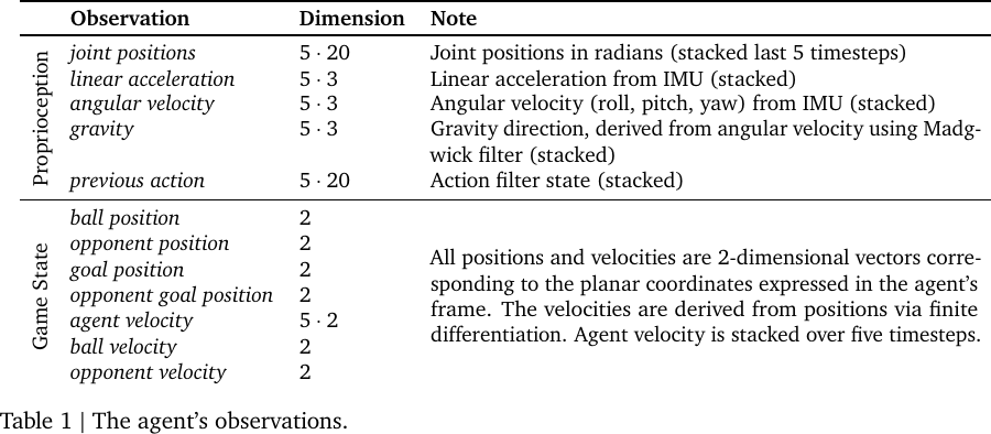
• State: In the real environment, the game state information is obtained via motion capture.

  Agent observation, from Table 1 of Tuomas Haarnoja et al., 2023.

  

• Action: A 20-dimensional continuous action that corresponds to the desired positions of the robot's joints. The action \(\va\) is sampled from a stochastic policy \(\pi(\cdot | \vh)\), where \(\vh\) is the observation-action history.

• Reward: The choice of reward function depends on the stage of training.

  Reward components, from Table 2 of Tuomas Haarnoja et al., 2023.

  

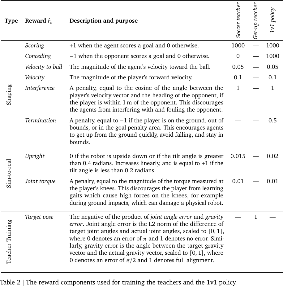
• Terminate Condition: In addition to the following conditions, the episode will terminate when reaching the horizon length.
  • Soccer Teacher: terminates when the agent falls over, goes out of bounds, enters the goal penalty area, or the opponent scores.
  • Get-up Teacher: terminates after reaching a target pose.
  • 1v1 Policy: terminates once a goal is scored.

2. Environment Setup

Environment Setup, from Figure 1 of Tuomas Haarnoja et al., 2023.

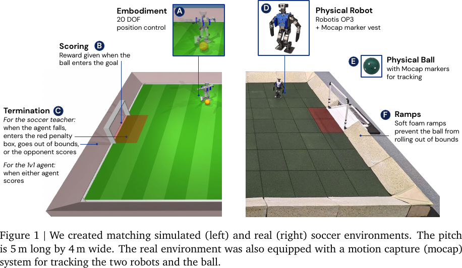
• Simulator: MuJoCo and DeepMind Control Suite.
• Robot Hardware: Robotis OP3
  • includes Logitech C920 webcam, which provide RGB video at 30 fps.
  • contains an inertial measurement unit (IMU), for providing angular velocity and linear acceleration data.
  • lacks GPUs, so the policy runs on CPU only.
  • added 3D-printed safety bumpers to reduce fall impact. Other minor modifications are also made to reduce the risk of breakages.
• Robot Software:
  • the servos are controlled with only proportional gain (i.e., no integral or derivative terms).
  • wrote a custom driver with the Dynamixel SDK Python API.
    • default driver was sometimes unreliable and caused indeterministic control latency.
• Motion Capture System:
  • 14 Optitrack PrimeX 22 Prime cameras with Motive 2 software.
  • captures robot and ball positions and orientations based on the markers attached to the robots' vest and the stickers on the ball.
  • data is streamed through wireless network through the VRPN protocol, and made available to the robots via ROS.

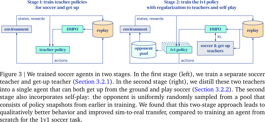
3. Two-stage Training

Two-stage Training, from Figure 3 of Tuomas Haarnoja et al., 2023.

1. Train teacher policies for two skills:

   • Soccer Teacher \(\pi_f(\cdot | \vh)\): Learn to score as much as possible against an untrained opponent. (that is, simply avoid the fallen opponent and score)

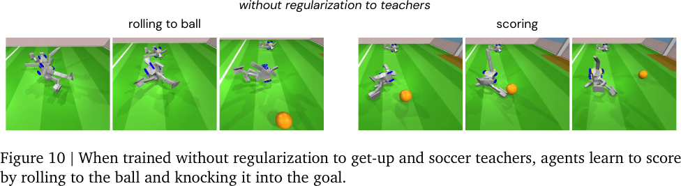
     • Terminating when falling over prevents the agent to find a local minimum and learn to roll on the ground towards the ball to knock it into the goal.

       Local minimum policy by rolling, from Figure 10 of Tuomas Haarnoja et al., 2023.

       

     • Training time: 158 hours. (\(2\cdot 10^9\) simulation steps)

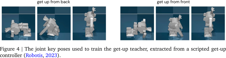
   • Get-up Teacher \(\pi_g(\cdot | \vh)\): Learn to get up from the ground.

     • Train to match a sequence of hand-crafted (scripted) target poses (joint angles and torso orientation), so as to learn a stable and collision-free trajectory, while not constraining the final behavior.

     • The agent learns to reach target poses gradually, starting with easier ones and progressing towards more challenging ones.

       The joint key poses used to train the get-up teacher, extracted from a scripted get-up controller, from Figure 4 of Tuomas Haarnoja et al., 2023.

       

     • Training time: 14 hours. (\(2.4\cdot 10^8\) simulation steps)

2. Train the 1v1 policy by maximizing:

   $$ J_\mathrm{total}(\pi)=\E_\vtau\left[\1_{\vs\in{\gU}}(J_{f}(\pi_{\theta})) + \1_{\vs\not\in{\gU}}(J_{g}(\pi_{\theta}))\right]$$

   • Distillation: Imitate (or regularized by) the two teacher policies.
     • \(\gU\) is the set of all states in which the agent is upright.
     • If the agent is upright (\(\vs\in{\gU}\)), regularize with the soccer teacher \(\pi_f(\cdot | \vh)\):
       $$ J_f(\pi_\theta)=(1-\lambda_f)\;J(\pi_\theta)-\lambda_f\E_\vtau\Big[\mathrm{KL}(\pi_\theta(\cdot|\vs)] \Vert \pi_f(\cdot|\vs))\Big]$$ If the agent is on the ground (\(\vs\not\in{\gU}\)), regularize with the get-up teacher \(\pi_g(\cdot | \vh)\):
       $$ J_g(\pi_\theta)=(1-\lambda_g)\;J(\pi_\theta)-\lambda_g\E_\vtau\Big[\mathrm{KL}(\pi_\theta(\cdot|\vs)] \Vert \pi_g(\cdot|\vs))\Big]$$
     • The weights \(\lambda_f,\lambda_g\in[0,1]\) are adaptively adjusted (from DiME) by minimizing: $$ c(\lambda)=\lambda(\E_\vtau[Q^{\pi_\theta}(\vs,\va)]-[\text{threshold}])$$ When the return \(Q\) surpasses the pre-defined threshold, \(\lambda\) decreases to 0 as the corresponding teacher is no longer needed.
     • \(J(\pi)\) is the expected discounted cumulative reward \(\E_\vtau\left[\sum\limits_{t=0}^T\gamma^t r(s_{t})\right]\).
   • Self-play: opponents are sampled from previous versions of the trained agent. (a form of automatic curriculum learning)
     • Sample policy snapshots only from the first quarter to improve stability. (from Neural Fictitious Self-Play and PSRO)
     • Condition the critic on the opponent ID is necessary since the value functions vary across opponents.
   • Maximize the RL objective with Distributional MPO (DMPO):
     • Actor \(\pi_\theta(\cdot | \vh)\): Maximum a Posteriori Policy Optimization (MPO), which outputs the mean and diagonal covariance of a multivariate Gaussian.
     • Critic \(Z^{\pi_\theta}_{\phi}(\vs, \va; [\text{opponent ID}])\): C51 (a distributional critic), which outputs a categorical distribution over Q-values.
   • Training time: 68 hours. (\(9\cdot 10^8\) simulation steps)

4. Sim-to-Real Transfer

• System Identification: Identify the actuator parameters
  1. Approximate with a position controlled actuator model with torque feedback.
     • Direct current control (that matches the servos' operating mode) doesn't transfer well to the real world.
  2. Apply a sinusoidal control signal of varying frequencies to a motor with a known load attached to it.
  3. Optimize over the actuator model parameters in simulation to match the resulting joint angle trajectory.
     • Only optimizes damping, armature, friction, maximum torque, proportional gain.
• Domain Randomization and Perturbations
  • Randomized the floor friction, joint angular offsets, varied the orientation and position of the IMU, and attached a random external mass to a randomly chosen location on the robot torso. Added random time delays to the observations, and applied random perturbations to the robot.
  • The values were resampled in the beginning of each episode, and then kept constant for the whole episode.
  • Selected a small number of axes to vary, since excess randomization could result in a conservative (worse) policy.
• Regularization for Safe Behaviors
  • Limit the joint range for preventing self-collision.
  • Penalize according to the time integral of torque peaks to prevent knee breakage during kicking.
  • Reward keeping an upright pose to avoid falling due to leaning too forward.

Experiments

Benchmark

Outperform scripted baselines quantitatively and qualitatively.

Analysis

• Visualize policy trajectories in three-dimensional space by Uniform Manifold Approximation and Projection (UMAP).

  Skill embeddings, from Figure 6 of Tuomas Haarnoja et al., 2023.

  

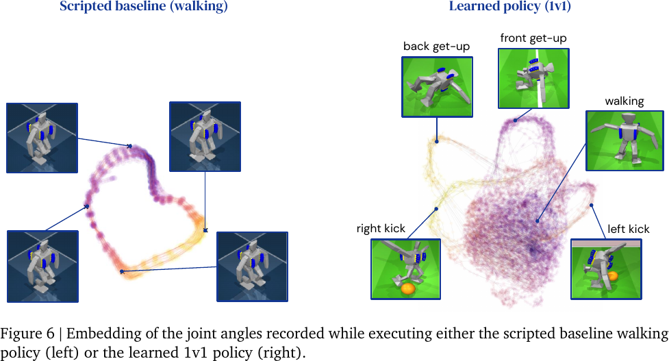
  • Scripted walking is based on periodic sinusoidal motions, so the gait is projected as a cyclic path.
  • The learned walking policy is richer, where the gait is projected as a dense ball.
  • The four topologically distinct loops corresponds to certain pre-trained or emergent skills.

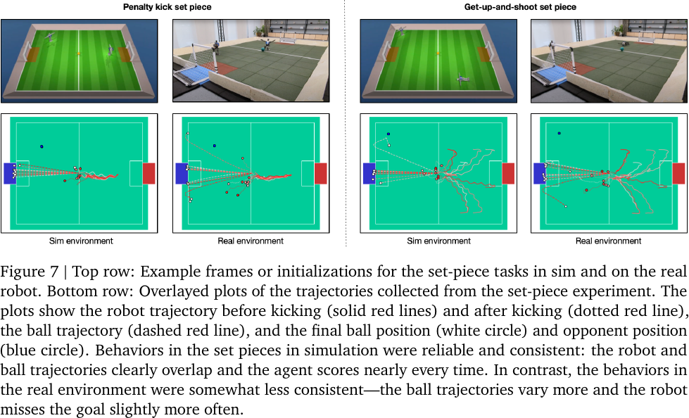
• Set Piece Analysis: state transitions in the real environment has higher variances, resulting in slight performance drop.

  Trajectories in simulation and real environment, from Figure 7 of Tuomas Haarnoja et al., 2023.

  

• Value Function Analysis: agent is sensitive to the observations of the ball, goal, and the opponent.

  Value function analysis, from Figure 8 of Tuomas Haarnoja et al., 2023.

  

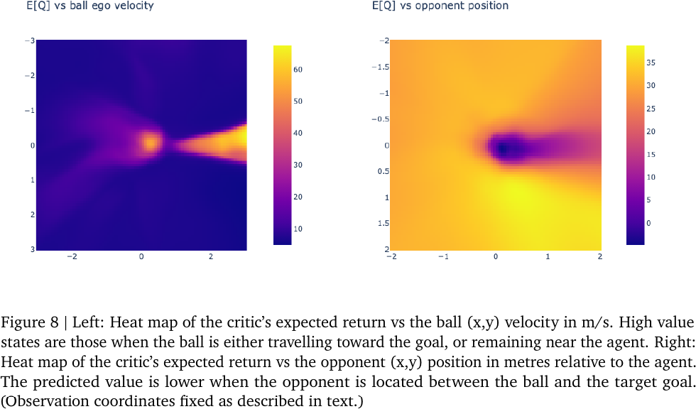
  • Robot agent is at the center \((0, 0)\), facing right.
  • The ball is in front of the robot, at \((0.1, 0)\).
  • The opponent is located at \((0, 1.5)\) in the left subfigure.

• Combination of skills: turning and moving toward the ball simultaneously.

  Adaptive footwork in a turn-and-kick set piece, from Figure 9 of Tuomas Haarnoja et al., 2023.

  

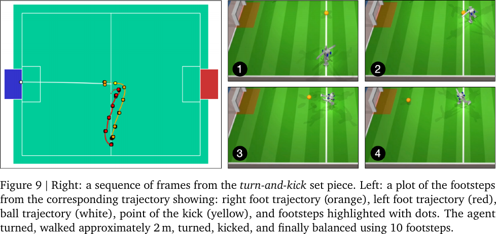
  • The agent is facing toward the opposite side of the ball.

Ablation Study

Run ablation studies on teacher regularization, sparse rewards, details of shape rewards, and self-play settings.

Playing Soccer from Raw Vision?

Playing soccer by only using onboard RGB camera and proprioception (IMU) introduces larger sim-to-real gap. Some preliminary experiments are conducted to investigate the feasibility of this setting.

• Create a visual rendering of the lab using a Neural Radiance Field (NeRF) model. (following NeRF2Real)
• Train multiple NeRF models with different background and lighting conditions, and randomly sample one during training.
• Combine the MuJoCo rendering of dynamic objects like the ball and opponent over the NeRF image, and randomizes the colors of the ball.
• Feed the superimposed image to an LSTM-based agent.

Official Resources

• Learning Agile Soccer Skills for a Bipedal Robot with Deep Reinforcement Learning [arxiv][site]

Comments