Autoregressive Models (AR/ARM)

$$ \def\pt{{p_\theta}} $$

Motivation: Factorizing the joint distribution into conditional 1D distributions to circumvent the need for modeling the (computationally expensive) joint distributions.

For example, consider a scenario involving \(D\)-dimensional data, where each dimension is defined by a categorical distribution with \(K\) categories. A total of \(K^D\) parameters are required to model the joint distribution, while only \(KD\) parameters are needed to model conditional 1D distributions.

Parameterization

Factorize the joint distribution to conditional 1D distributions by chain rule of probability: $$ p(\vx) = p(\vx_{1:D}) = p(x_1,\dots,x_D) = p(x_1)p(x_2|x_1)p(x_3|x_2,x_1)\dots = \prod_{i=1}^D p(x_i|\vx_{<i}) $$

where \(\vx_{<i} = \vx_{1:i-1}\).

Connection to RNNs

The condition of each term \(p(x_i|\vx_{<i})\) becomes more complex as \(i\) increases. This issue can be mitigated by:

• (first-order) Markov assumption: \(p(x_i|\vx_{<i}) = p(x_i|\vx_{i-1})\), or
• Hidden Markov model (HMM): \(p(x_i|\vx_{<i}) = p(x_i|\vz_{i-1})\), where \(\vz_{i-1}\) contains the compressed information of \(\vx_{<i}\).
  • Under the special case that \(\vz_i\) is a deterministic function (instead of a stochastic funcion) of \(\vz_{i-1}\), the model correpsonds to RNNs.

The conditionals \(p(x_i|\vx_{<i})\) can be modeled by the following:

• Discrete distributions
  • Categorical distributions: parameterized by \(K\) categories \(\vp_i\in[0,1]^K\): $$ p(x_i|\vx_{<i}) = \prod_{k=1}^K p_{i,k}^{[x_i=k]} $$
• Continuous distributions
  • (Mixture of) Gaussians: parameterized by \(K\) gaussians \([(\mu_{i,k}, \sigma_{i,k}, \alpha_{i,k})]_{k\in\{1,\cdots,K\}}\): $$ p(x_i|\vx_{<i}) = \sum_{k=1}^K \alpha_{i,k}\ \gN(x_i | \mu_{i,k}, \sigma_{i,k}) $$
  • Cumulative distributions: autoregressive implicit quantile networks (AIQN), and etc.

In practice, while we only define the model architecture of \(p(x_i|\vx_{<i})\) in code, the full model can be perceived as a deep architecture comprising \(D\) layers of \(p(x_i|\vx_{<i})\).

Pointwise Evaluation

• Pointwise evaluation of \(\pt(\vx)\)?

  • Yes, as long as \(\pt(x_i|\vx_{<i})\) is modeled as a distribution that can be easily evaluated.
  • Simply compute \(\pt(\vx) = \prod_{i=1}^D \pt(x_i|\vx_{<i})\).

Data Generation

• Generating new samples \(\rvx\sim\pt(\vx)\)?

  • Yes, as long as \(\pt(x_i|\vx_{<i})\) is modeled as a distribution that can be easily sampled from, and \(\pt\) doesn't overfit.
  • Sample each dimension autoregressively \(\rvx_i\sim \pt(x_i|\vx_{<i})\), and concatenate the output after \(D\) forward passes (slow, one forward pass for each conditional).

• Conditional generation \(\rvx\sim\pt(\vx|\vc)\)?

  • Yes, simply define \(\vc=\vx_{1:C}\) (i.e., a prompt), where \(\vc\in\R^C\) and \(D_\mathrm{new}=D+C\).

• Imputation \(\rvx_m\sim\pt(\vx_m|\vx_o)\)?

  • No in general, not for causal ARs. May require more advanced ARs such as bi-directional ARs (e.g., BERT, BAT-Fill)

Training Target

We need to derive \(\nabla_\theta\log\pt(\rvx)\) to perform Maximum Likelihood training (as shown in Maximum Likelihood Estimation):

\[ \begin{aligned} \log\pt(\rvx) &= \log \pt(\rx_1, \dots, \rx_D) \\ &= \log\prod_{i=1}^D \pt(\rx_i|\rvx_{<i}) \\ &= \sum_{i=1}^D \log\pt(\rx_i|\rvx_{<i}) \\ \end{aligned} \]

The Negative Log-Likelihood (NLL) loss function is defined as: $$ L(\theta) = \E_{\rvx\sim\ptrain(\vx)}[-\sum_{i=1}^D \log\pt(\rx_i|\rvx_{<i})] $$

which can be optimized based on its gradients: $$ \nabla_\theta L(\theta) = \E_{\rvx\sim\ptrain(\vx)}[-\sum_{i=1}^D \nabla_\theta\log\pt(\rx_i|\rvx_{<i})] $$

Examples

PixelCNNs

Visualization of conditional distributions, from Figure 2 of Oord et al., 2016.

• For images, \(\pt(\vx): \{0,\dots,255\}^{HWC} \to \R^{HWCK}\).
  • The pixels of the image are ordered sequentially by concatenating the rows: \([\text{row 1}, \text{row 2}, \dots]\) (i.e., raster scan ordering).
  • The color channels are ordered sequentially by concatenating the RGB values: \([r, g, b]\).
  • Every \(\pt(x_i|\vx_{<i})\) is modeled by a categorial distribution with support \(\{0,\dots,255\}\) (i.e., \(K=256\)), where each category corresponds to the color intensity of the channel.
• Code implementation:
  • Output as categorical distribution: See the low and high parameters in the TensorFlow implementation, or the PixelCNN(pl.LightningModule) module in phlippe/uvadlc_notebooks.
    • The output of the model lies in \(\mathbb{R}^{HWCK}\), indicating a conditional categorical distribution represented in \(\mathbb{R}^K\) for each pixel color.
  • Output as binary categorical distribution: When the data only contains black-and-white images, the output shape can be the same as the input shape to save parameters, as in the Keras implementation or in EugenHotaj/pytorch-generative.
    • Please note that this technique only works under the special case where the data contains binary values.
  • Sampling: See the def sample function in phlippe/uvadlc_notebooks.

(Generative) Transformers

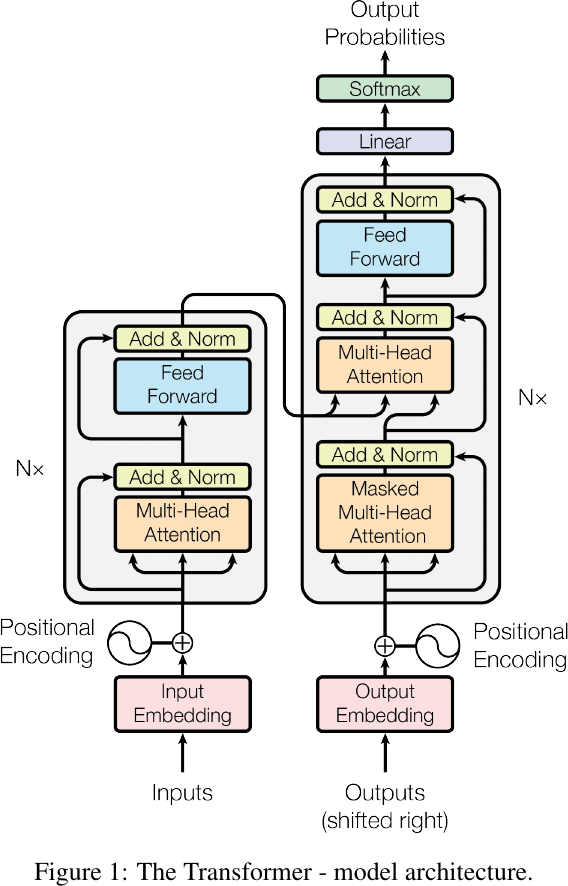
The Transformer model architecture, from Figure 1 of Ashish Vaswani et al., 2017.

• For natural language processing, \(\pt(\vx): \{1,\dots,K\}^{D} \to \R^{DK}\) (for simplicity, we assume the I/O shares the same tokenizer and operate on token level).
  • Every \(\pt(x_i|\vx_{<i})\) is modeled by a categorial distribution with support \(\{1,\dots,\text{vocab size}\}\) (i.e., \(K = \text{vocab size}\)), where each category corresponds to the index of a token in the vocabulary.
  • The vocabulary size depends on the tokenizer used. For example, the GPT-2 tokenizer has a vocabulary size of 50,257.
• Code implementation:
  • Dimensions of input \(\vx\): See the Embeddings(nn.Module) module in harvardnlp/annotated-transformer.
    • Please note that nn.Transformer in PyTorch works in embedding space. An extra nn.Embedding lookup operator followed by a PositionalEncoding is required to map the input to embedding space.
  • Categorical distribution: See the Generator(nn.Module) module in harvardnlp/annotated-transformer.
    • Please note that nn.Transformer in PyTorch works in embedding space. An extra nn.Linear layer and log-softmax operator is required to map the output from embedding space to the vocabulary distribution.
    • The output of the model lies in \(\mathbb{R}^{DK}\), indicating a conditional categorical distribution represented in \(\mathbb{R}^K\) for each token.
  • Sampling: See the def greedy_decode part in harvardnlp/annotated-transformer, or the for i in range(args.words) part in pytorch/examples.
• The overall inference process from an application viewpoint involves the following steps:
  • The input text (character sequence) is tokenized into tokens (character/byte sequences), which are then mapped to token IDs (integers). These token IDs are further transformed into a sequence of embeddings (vector sequence).
  • After that, the vector sequence is input into the Transformer model, producing another sequence of embeddings (vector sequence), which in turn are transformed into logits (number sequence).
  • Lastly, the logits are normalized into a sequence of probabilities (number sequence) by the softmax operator, which can be used to sample the next token ID (integer) of the output sequence. This sampling process can be repeated to generate a sequence of token IDs (integer sequence), which can be mapped back to tokens (character/byte sequences), ultimating yielding the final output text (character sequence).

Community Resources

•  Probabilistic Machine Learning: Advanced Topics (i.e., probml-book2)
  • Chapter 22: Auto-regressive models

Comments